The shape of the demand curve depends on two forces: the substitution effect and the income effect. A typical treatment:
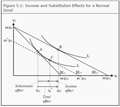
When the price of q1, p1, changes there are two effects on the consumer. First, the price of q1 relative to the other products (q2, q3, . . . qn) has changed. Second, due to the change in p1, the consumer’s real income changes.
In case that’s not instantly clear, intermediate microeconomics textbooks graphically decompose the two effects for consumers choosing between two goods:
While there’s nothing incorrect about the preceding text or figure, they’re unlikely to make the typical undergraduate say, “Aha! I get it.” Most students readily grasp the substitution effect: If the price of x goes up, you’ll naturally cut back on x. How can teachers make the income effect just as obvious?
My answer: Instead of poring over the standard two-good choice problem to decompose the substitution and income effects, teachers should start with a one-good choice problem. In this one-good setting, there is plainly no substitution effect; there is nothing to substitute to. Yet quantity demanded still clearly depends on price. If you have $50 to spend, and the price of the only good jumps from $10/unit to $25/unit, consumers reduce their consumption from 5 units to 2 units. Why? There’s only one possibility: When the price goes up, the consumer’s real income automatically goes down. That, students, is an unadulterated income effect.
Once students see an income effect without a substitution effect, many professors will want to show them a substitution effect without an income effect. Soon they’ll be patiently explaining the income-compensated demand curve – and once again losing most of their audience. A better approach: Posit a consumer choosing between a thousand different goods, none of them a large fraction of the budget. If the price of a single good rises, the effect on the consumer’s real income is negligible. But consumers will still respond to the rising price of x by buying less x.
My one-good and thousand-good problems lead straight to the meaty question: When is the income effect important, and when can it be safely ignored? With only one good, the income effect is all-important. With many goods, each a small share of the budget, the income effect is trivial. So when is the income effect important without being all-important? When at least one good is a sizable chunk of the budget, without being the whole tamale.
Housing is a great example. Most students will instantly see that a 10% rise in their rent will make them feel poorer across the board. And once students concede this point, it’s fairly easy to convince them that leisure fits the mold at well. Backward-bending labor supply curves, here we come.
What about the math and the graphs? Frankly, if your students aren’t going to graduate school, I’d skip both. But if that’s too radical, you should still begin with my approach. Make sure your students have the underlying intuitions firmly in mind. Then show them the traditional way of formalizing those intuitions. If you must bore your students into a stupor, at least teach them some economics first!
READER COMMENTS
Brian Albrecht
Sep 2 2014 at 11:01pm
I’ve already filed this away for later this semester.
Also, I’d love more posts about teaching these concepts.
Wayward
Sep 2 2014 at 11:17pm
Thank you if you have time please do more for us non-students.
David Flath
Sep 2 2014 at 11:26pm
I disagree. In my experience it’s the substitution effect that students don’t get.
Students think the law of demand reflects an income effect: “If price goes up I can’t afford as much and so buy less.” They don’t think in terms of a substitution effect at all (and imagine all goods are normal. The Alchian oranges example illustrates the substitution effect, and its close relation to the law of demand, and that is what economics students really need to learn. What do you think?
Alex Tabarrok
Sep 2 2014 at 11:50pm
Another possibility, instead of a thousand goods for the substitution effect try zero. That is, choose a good that you currently don’t buy, say cashmere sweaters. Suppose the price of cashmere sweaters falls–there is no income effect since your current spending on cashmere sweaters is zero but at some low price you might buy a cashmere sweater–that’s the substitution effect.
David R. Henderson
Sep 3 2014 at 9:52am
@David Flath,
Good point. BTW, great to hear from you after all these years. To others: David was in graduate school with me in the early 1970s to mid-1970s.
@Alex,
Very clever. Thanks.
roystgnr
Sep 3 2014 at 9:59am
Are there any estimates for how far that labor supply curve bends back? Leisure becomes more valuable as you find yourself with less of it, but it never becomes *infinitely* valuable… Money becomes less valuable as you find yourself with more of it, but even the ultra-rich often seem to enjoy accumulating more to give to charity or to their kids.
Todd Kreider
Sep 3 2014 at 5:14pm
David Flath also wrote a very good text on the Japanese economy, which I see has a 2014 third edition.
Since discussing income here, there is an interesting error on p.18 with respect to cross country comparisons of the gini coefficient that has been often repeated in the Japan field.
I think the error arises because a World Bank 2002 report table was reproduced showing Japan had a gini coefficient of .25 in 1993 with the U.S. at .41, showing that twenty years ago Japan was much more equal compared to the U.S. and based on more recent numbers that Japan’s inequality has jumped significantly.
But this is an apples to oranges comparison error if Tachibanaki’s government data is correct in Confronting Economic Inequality in Japan is correct.
He has a table on p.4 that shows Japan had a post-transfer gini coefficient of .37 in 1993 and .38 in 2002. (This has hardly changed over the past decade. The next table on p.5 is from the OECD
that shows a household adjusted gini coefficient of .31 for Japan and .34 for Japan in for 1995 to 1996. [Both pages can be viewed through Amazon]
Japan’s post-transfer inequality was always somewhat less than that of the U.S. since at least the 1980s but never close to the .25 versus .41 gap reproduced in Flath’s text.
Steve Horwitz
Sep 3 2014 at 7:30pm
I think students get this distinction the best by just teaching the backward bending labor supply curve FIRST. Once they get the idea that an increase income allows them to purchase more leisure even as the rising opportunity cost of leisure induces less of it purchased, I think they can get it on the demand curve side. YMMV of course.
William Polley
Sep 4 2014 at 10:22am
I try to emphasize that the income and substitution effects are two forces acting in the same or different directions. We observe the result (or resultant vector, for the scientifically inclined) but do not observe the individual forces directly. Then I show a YouTube video of a jumbo jet landing in a crosswind to illustrate a physical example of opposing forces.
I also wrote a Mathematica demonstration that illustrates income and substitution effects.
Lauren Heller
Sep 8 2014 at 1:35pm
Another fun thing I do when teaching income effects (in contrast to substitution effects) is to use this State Farm commercial:
https://m.youtube.com/watch?v=sUVJ9MCfZvY
Basically, the gist is that when the price of insurance decreases, the customer has more income with which to purchase EVERYTHING (including falcons!). It just helps me add some levity to what can sometimes be a (gasp!) slightly boring topic.
Kristian Niemietz
Sep 12 2014 at 5:37pm
I used the price of a seasonal ticket for the underground to illustrate a situation in which the income effect dominates, and the price of a coffee in the student cafeteria to illustrate a situation in which the substitution effect dominates. Did it work? Well, fewer blank faces than when I just drew the graph.
Comments are closed.